Foreword

- Most of the things you need to think about are described in the OHBM MEEG COBIDAS.

Brain in numbers

The cerebral cortex is composed of 3 cortices with different phylogenetic origins:

- the paleocortex (1% of the cortical surface, mainly olfactif cortex)

- the archicortex (3-4% of the cortical surface, hippocampic region)

The neocortex (95% of the cortical surface, 6 layers organization, 32% frontal cortex, 30% parietal cortex, 23% temporal cortex and 15% occipital cortex). The whole cerebral cortex volume is around 300cm^3 for men and 270cm^3 for women. The cortical surface represents 2200cm^2 and the neocortex thickness varies from 1.5 to 4.5mm.

Blood flow and Metabolism

An average brain weights about 1400g, i.e. only 2 to 3% of the total body weight. The air entering our lungs contains 21% oxygen, and by the time the oxygen reaches our brain this value has fallen to 4%. Yet, an adult brain consumes about 20% of the whole blood oxygen and about 750mL of blood every minute, extracting 10% of the 90mg/dL of glucose contained in the blood.

Neurons

The estimated number of neuron varies between 2.6x10^9 and 16x10^9, with a density of 14-18 neurons in the agranular cortex to 40-100 neurons for 0.001mm^3 in the visual cortex. Despite this huge numbers, neurons make up only 10% of brain cells and about 90% of the cells are glial (microglia, astrocytes, oligodendrocytes). One neuron may have hundreds or thousands of synapses on its dendrites and soma and the estimated number of synapses is 100x10^12 synapses for the human brain. For an average 55mm cubic voxel, less than 3% of the volume is occupied by vessels and the rest by neural elements. This means that in an unfiltered (smoothed) voxel there is about 5.5 million neurons, 2.2^10 to 5.5^10 synapses, 22 km of dendrites and 220 km of axons (Logothetis, Nature 453, 2008)

ElectroPhysiological Recording

Neuronal Recording

An EPSP that reaches an apical dendrite activates non-specific cation channels and thus elicits a depolarization of the cell membrane. The variation of the electrical potential depends of the importance of the EPSP and the resistivity of the membrane (highest resistivity if numerous IPSP). For intracellular recording, the electrical potential relies on the comparison between the membrane cell and the extracell environment. Thus, the variation of the electrical potential reflects roughly the product of the importance of EPSP by the resistivity. If we use an electrode in the extracellular environment (extracell recording) but close to cell, the variation of the electrical potential will depend on the importance of EPSP and the resistance of the extracellular environment. One difference is the amplitude of the response, intracell recording shows membrane depolarization and thus the amplitude is in millivolt, whereas for extracell recording, the amplitude is in microvolt. But, most important, the intracell recording signal is always positive whereas the extracell recording shows different polarities according to the electrode position. If the electrode 'looks' at where current enters, the signal is negative, whereas if it looks at where the current leaves, the signal is positive.

A manoelectrode located on the cortex record field potentials, i.e. the sum of extracell potentials elicited by the synchronous firing of neurons. Field potentials varies according to, at least, 4 characteristics:

i) the amplitude decreases according to the distance (1/d^2) between the electrode and the neural population.

ii) when EPSP arrive to the surface layers, the electrode see positive charges 'leaving' and thus record a negative potential, whereas a deep electrode see positive charges 'approaching' and this record a positive potential and vis versa when EPSP arrive to the deep layers.

iii) polarities are reversed for IPSP.

iv) it exist a continuum between surface and deep electrodes.

MEG/EEG

The electrical activity of neuronal populations, and thus magnetic concurrent fields, can be recorded using macro-detectors on the scalp surface. One can distinguish primary currents, which are related to the movement of ions, and volume currents that correspond to passive ohmic currents settled up in the surrounding medium. Recorded variations correspond to the sum of ionic current in the extracellular space.

EEG

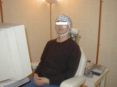
The ElectroEncephalography method measures neuronal activity using several electrodes placed on the scalp (fig 1). EEG recording corresponds to the electrical potential difference between two electrodes: either between one active electrode on the scalp and one reference electrode located far from the recording site, or between two active electrodes. Amplitudes (20 to 100 microvolt) and frequencies (1 to 40hz) vary according to subjects' activity. According to the position of electrodes and cortical current, the signal can be positive or negative.

MEG

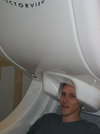
The fluctuating electrical currents measured with EEG also produce a magnetic field over the head. Because the same neuronal population elicits EEG and MEG components, both techniques measure roughly the same thing. However, MEG spatial maps are quite different and techniques are more complementary than redundant (see "neural sources"). Looking at map patterns, one can see that EEG and MEG tend to present perpendicular patterns due to the difference in the type of sources. The measured neuromagnetic field is extremely weak, about 10^-12 tesla, which is weaker than the urban's magnetic background (10^-7 T) and the earth's magnetic field (10^-4 T). Therefore, in contrast with EEG, MEG measurements need a suppression of any fluctuating magnetic background and highly sensitive detectors. The suppression of the fluctuating magnetic background is performed by the use of a shielded room (exclude external magnetic fields) and a measure of magnetic gradient within the shielded room. Detectors are complex coils (SQUID Superconducting Quantum Interference Device) that measure the weak magnetic fluxes. One can roughly summarize the concept of a SQUID as a superconduction ring interrupted by two Josephson junctions that limit the flow of the supercurrent, making easier to exploit flux quantization for the measurement of the magnetic field. The magnetic flux is measured through the SQUID loop since current over the Josephson's junctions is a periodic function of this magnetic flux. Measures are based on the fact that the voltage over the junctions is approximately a linear function of the magnetic flux. The signal is carried to SQUID via a flux transformer. A flux transformer is also a superconducting loop. Thus, magnetic fluxes induce a current in it that is a direct function of the magnetic density, with no signal loss. Modern MEG devices uses several transformers for a given locations, usually one for the x direction and one for the y direction perpendicular to z magnetic flux, which is the magnetic flux perpendicular to the surface of the helmet.

Neural Sources

If the primary source and the surrounding conductivity distribution are known, the resulting electric potential and magnetic fields can be calculated from Maxwell's equations. Looking at EEG or MEG data is known as the electromagnetic inverse problem, i.e. dealing with the deduction of the source currents responsible for the measured field. Indeed, such problem has no unique solution (von Helmholtz, 1853) and source models are used to approximate the solution. The optimal solution is usually found by fitting (least-squares method) the theoretical and measured field patterns to get the equivalent current dipole (ECD).

Both EEG and MEG provide a projection of primary current distribution on the respective lead fields, i.e. the sensitivity distribution of the detectors, and measure weighted integrals of this primary current distribution. In general, MEG gives a better spatial information than EEG. First, MEG is sensitive to dipoles oriented radially to the skull only. This is due to the symmetry and cancellations that take place in perfectly spherical conductors (of course in the real word, the head of our subjects is not perfectly spherical) and there is only one MEG signal for a tangential dipole. Second, EEG measures both radial and tangential sources leading to more complex interpretation of the sources. Indeed, because tangential electrical sources tend to be located in the sulci and radial one on the gyri, MEG and EEG are complementary techniques for a full investigation of neural sources. And third, the electrical lead field is affected by the conductivity of the skull and the scalp leading to blurred signal whereas the magnetic field is not altered by such inhomogeneities.

For a full review of mathematical methods on the direct and inverse problem as well as a full description of MEG device see: Hämäläinen, M., Hari, R., Limoniemi, R.J., Knuutila, J. & Lounasmaa, O.V. (1993). Magnetoencephalography - theory, instrumentation, and applications to noninvasive studies of the working human brain. Reviews of Modern Physics, 65, 413-497.

Electrophysiology Statistics

The LIMO project

The LInear MOdelling toolbox, is a matlab based code aiming at providing full sensor or source space analysis of your EEG or MEG data. It is 100% compatible with EEGLAB for which we have a STUDY GUI integration, and the code is also compatible with FieldTrip (at least for ERP). See out GitHub repository for more information.

Multiple comparison corrections in MEEG

As part of the LIMO tools, corrections for false positives need to be developped given the huge number of statistical tests we perform. You can learn about this topic in this blog post.